Validation
Singlephase flow
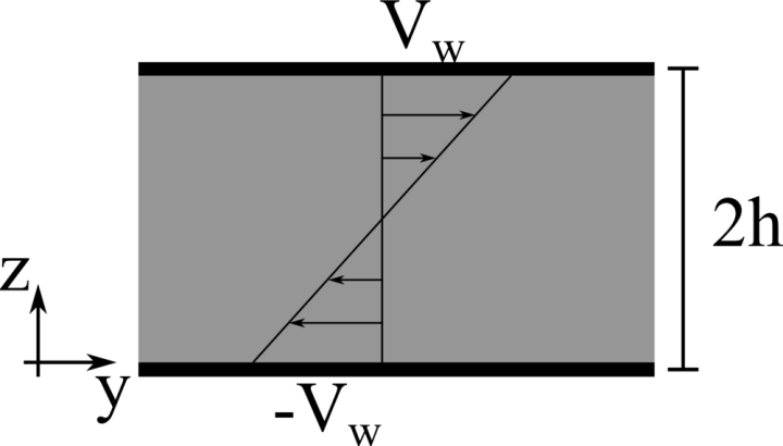
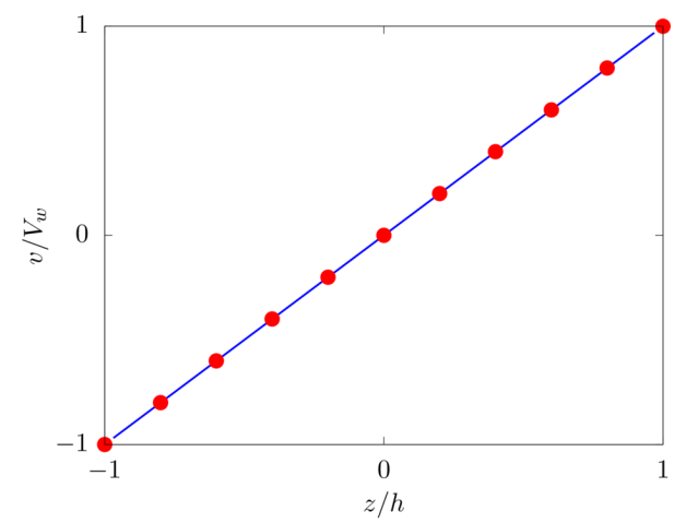
Laminar plane Couette flow
Analytical solution: \(v \left( z \right) = -V_w \left( 1-z/h \right)\).
config.h
#define _FLOW_COUETTE_
#define _FLOW_INIT_LAMINAR_
#define _SOLVER_FFT2D_
#define _SINGLEPHASE_
parameters.f90
! Total number of grid points in X, Y and Z
integer, parameter :: nxt = 4, nyt = 4, nzt = 32
! Size of the domain in X, Y and Z
real, parameter :: lx = 0.25, ly = 0.25, lz = 2.0
! Fluid viscosity and density
real, parameter :: vis = 0.1, rho = 1.0
! Reference velocity (bulk velocity or wall velocity)
real, parameter :: refVel = 1.0
! Gravitational acceleration
real, dimension(3), parameter :: gr=(/0.0,0.0,0.0/)
input/input.in
# Simulation initial and final steps
0 100
# Simulation initial time
0.0
# Simulation initial time-step
0.0002
# Output frequency: 0D, 1D, 2D, 3D, restart data
100 100 100 1000000 1000000
# Simulation restart condition for the multiphase part
.false.
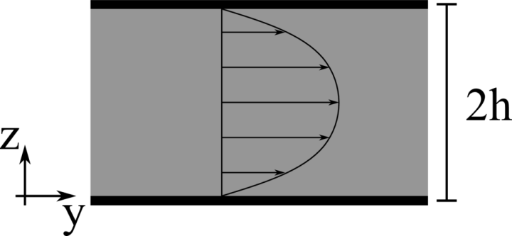
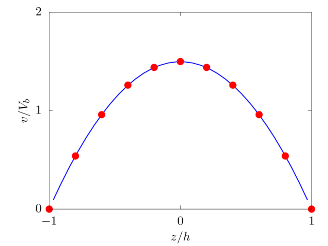
Laminar plane Poiseuille flow
Analytical solution: \(v \left( z \right) = 6 V_b \left( z/2h \right)\left[ 1- \left( z/2h \right) \right]\).
config.h
#define _FLOW_CHANNEL_
#define _FLOW_CHANNEL_CFR_
#define _FLOW_INIT_LAMINAR_
#define _SOLVER_FFT2D_
#define _SINGLEPHASE_
parameters.f90
! Total number of grid points in X, Y and Z
integer, parameter :: nxt = 4, nyt = 4, nzt = 32
! Size of the domain in X, Y and Z
real, parameter :: lx = 0.25, ly = 0.25, lz = 2.0
! Fluid viscosity and density
real, parameter :: vis = 0.1, rho = 1.0
! Reference velocity (bulk velocity or wall velocity)
real, parameter :: refVel = 1.0
! Gravitational acceleration
real, dimension(3), parameter :: gr=(/0.0,0.0,0.0/)
input/input.in
# Simulation initial and final steps
0 100
# Simulation initial time
0.0
# Simulation initial time-step
0.0002
# Output frequency: 0D, 1D, 2D, 3D, restart data
100 100 100 1000000 1000000
# Simulation restart condition for the multiphase part
.false.
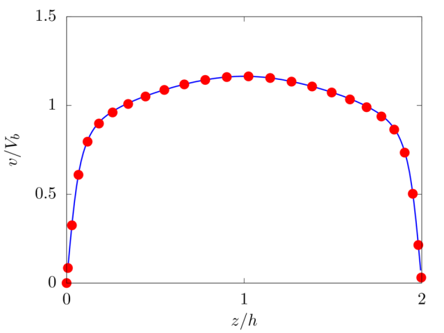
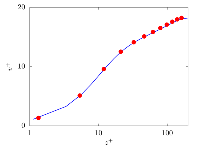
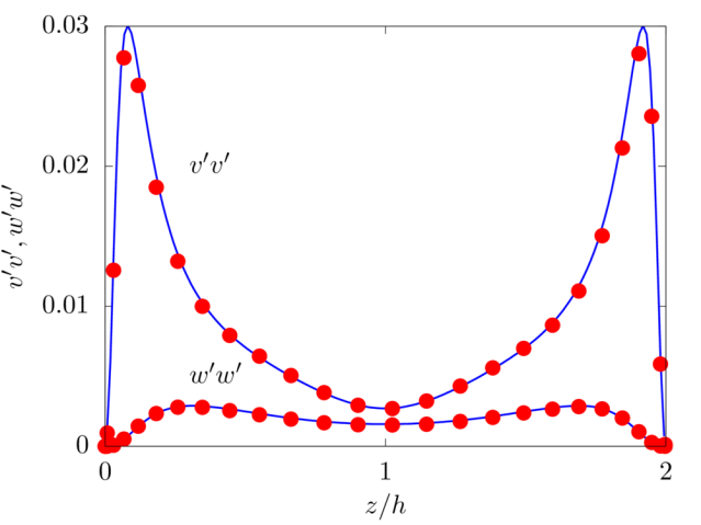
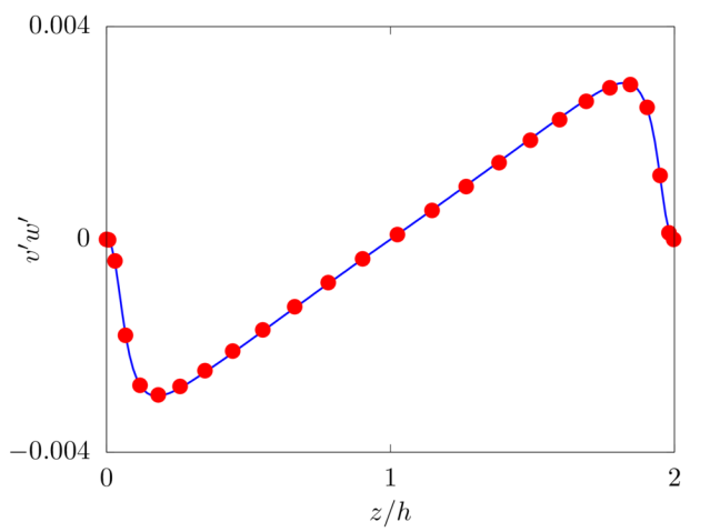
Turbulent plane channel flow
config.h
#define _FLOW_CHANNEL_
#define _FLOW_CHANNEL_CFR_
#define _FLOW_INIT_TURBULENT_
#define _SOLVER_FFT2D_
#define _SINGLEPHASE_
parameters.f90
! Total number of grid points in X, Y and Z
integer, parameter :: nxt = 256, nyt = 512, nzt = 160
! Size of the domain in X, Y and Z
real, parameter :: lx = 3.0, ly = 6.0, lz = 2.0
! Fluid viscosity and density
real, parameter :: vis = 2.0/5600.0, rho = 1.0
! Reference velocity (bulk velocity or wall velocity)
real, parameter :: refVel = 1.0
! Gravitational acceleration
real, dimension(3), parameter :: gr=(/0.0,0.0,0.0/)
input/input.in
# Simulation initial and final steps
0 9999999
# Simulation initial time
0.0
# Simulation initial time-step
0.002
# Output frequency: 0D, 1D, 2D, 3D, restart data
100 1000 2000 1000000 10000
# Simulation restart condition for the multiphase part
.false.
ABC flow
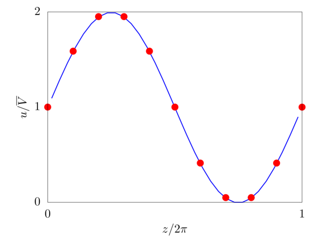
We consider the Arnold-Beltrami-Childress (ABC) flow in a three-periodic domain of size \(2\pi L\). The velocity field is initialized as
\(u = \overline{V} \left[ \sin \left( z/L \right) + \cos \left( y/L \right) \right],\)
\(v = \overline{V} \left[ \sin \left( x/L \right) + \cos \left( z/L \right) \right],\)
\(w = \overline{V} \left[ \sin \left( y/L \right) + \cos \left( x/L \right) \right].\)
The Reynolds number \(Re = \rho \overline{V} L /\mu\) is fixed equal to \(10\) and \(32\) grid points per side are used to discretise the numerical domain.
config.h
#define _FLOW_TRIPERIODIC_
#define _FLOW_TRIPERIODIC_ABC_
#define _FLOW_INIT_LAMINAR_
#define _SOLVER_FFT3D_
#define _SINGLEPHASE_
parameters.f90
! Total number of grid points in X, Y and Z
integer, parameter :: nxt = 32, nyt = 32, nzt = 32
! Size of the domain in X, Y and Z
real, parameter :: lx = 2.0*acos(-1.), ly = 2.0*acos(-1.), lz = 2.0*acos(-1.)
! Fluid viscosity and density
real, parameter :: vis = 0.1, rho = 1.0
! Reference velocity (bulk velocity or wall velocity)
real, parameter :: refVel = 1.0
! Gravitational acceleration
real, dimension(3), parameter :: gr=(/0.0,0.0,0.0/)
input/input.in
# Simulation initial and final steps
0 100
# Simulation initial time
0.0
# Simulation initial time-step
0.0002
# Output frequency: 0D, 1D, 2D, 3D, restart data
100 100 100 1000000 1000000
# Simulation restart condition for the multiphase part
.false.
Taylor-Green Vortex
We consider the time evolution of a Taylor-Green vortex in a three-periodic domain of size \(2\pi L\). The velocity field is initialized as
\(u = U \sin \left( x/L \right) \cos \left( y/L \right) \cos \left( z/L \right),\)
\(v = -U \cos \left( x/L \right) \sin \left( y/L \right) \cos \left( z/L \right),\)
\(w=0.\)
The Reynolds number \(Re = \rho U L /\mu\) is fixed equal to \(1600\) and \(512\) grid points per side are used to discretise the numerical domain.
config.h
#define _FLOW_TRIPERIODIC_
#define _FLOW_TRIPERIODIC_TGV_
#define _FLOW_INIT_LAMINAR_
#define _SOLVER_FFT3D_
#define _SINGLEPHASE_
parameters.f90
! Total number of grid points in X, Y and Z
integer, parameter :: nxt = 512, nyt = 512, nzt = 512
! Size of the domain in X, Y and Z
real, parameter :: lx = 2.0*acos(-1.), ly = 2.0*acos(-1.), lz = 2.0*acos(-1.)
! Fluid viscosity and density
real, parameter :: vis = 1.0/1600.0, rho = 1.0
! Reference velocity (bulk velocity or wall velocity)
real, parameter :: refVel = 1.0
! Gravitational acceleration
real, dimension(3), parameter :: gr=(/0.0,0.0,0.0/)
input/input.in
# Simulation initial and final steps
0 9999999
# Simulation initial time
0.0
# Simulation initial time-step
0.0002
# Output frequency: 0D, 1D, 2D, 3D, restart data
100 1000000 1000000 1000000 10000
# Simulation restart condition for the multiphase part
.false.
Homogeneous Isotropic Turbulence
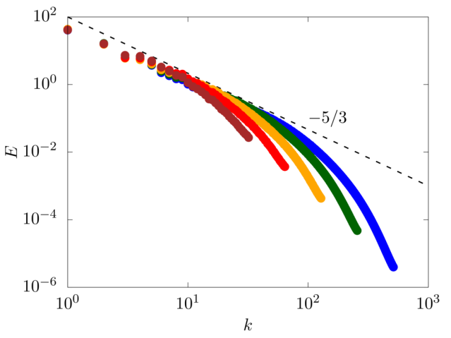
We consider an homogeneous isotropic turbulent flow in a three-periodic domain of size \(2\pi L\). The flow is sustained by a random forcing in Fourier space [4] on wave numbers within a shell of radius \(k=2\). The Taylor microscale Reynolds number \(Re = \rho u' \lambda /\mu\) is varied from \(100\) to \(400\), and \(64\), \(128\), \(256\), \(512\) and \(1024\) grid points per side are used to discretise the numerical domain.
config.h
#define _FLOW_TRIPERIODIC_
#define _FLOW_TRIPERIODIC_ISO_
#define _FLOW_INIT_LAMINAR_
#define _SOLVER_FFT3D_
#define _SINGLEPHASE_
parameters.f90
! Total number of grid points in X, Y and Z
integer, parameter :: nxt = 1024, nyt = 1024, nzt = 1024
! Size of the domain in X, Y and Z
real, parameter :: lx = 2.0*acos(-1.), ly = 2.0*acos(-1.), lz = 2.0*acos(-1.)
! Fluid viscosity and density
real, parameter :: vis = 1.0/400.0, rho = 1.0
! Reference velocity (bulk velocity or wall velocity)
real, parameter :: refVel = 1.0
! Gravitational acceleration
real, dimension(3), parameter :: gr=(/0.0,0.0,0.0/)
input/input.in
# Simulation initial and final steps
0 9999999
# Simulation initial time
0.0
# Simulation initial time-step
0.00001
# Output frequency: 0D, 1D, 2D, 3D, restart data
100 1000000 1000000 1000000 10000
# Simulation restart condition for the multiphase part
.false.
References:
[1] D. S. Henningson and J. Kim. On turbulent spots in plane poiseuille flow. Journal of Fluid Mechanics, 228:183–205, 1991.
[2] J. Kim, P. Moin, and R. Moser. Turbulence statistics in fully developed channel flow at low Reynolds number. Journal of Fluid Mechanics, 177:133–166, 1987.
[3] W. M. Van Rees, A. Leonard, D. I. Pullin, and P. Koumoutsakos. A comparison of vortex and pseudo- spectral methods for the simulation of periodic vortical flows at high reynolds numbers. Journal of Computational Physics, 230(8):2794–2805, 2011.
[4] V. Eswaran and S. B. Pope. An examination of forcing in direct numerical simulations of turbulence. Computers & Fluids, 16(3):257–278, 1988.
VOF
Buoyancy-driven flow
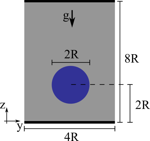
We consider a 2D droplet of radius \(R\) rising in a fluid with different density and viscosity. The droplet has viscosity \(\mu_1\) and density and \(\rho_1\), while the surrounding fluid has viscosity \(\mu_2\) and density \(\rho_2\), providing a viscosity and density ratio equal to \(k_\mu = 10\) and \(k_\rho = 10\). The two fluids are separted by an interface with interfacial surface tension \(\sigma\). The domain is rectangular with size \(4 R \times 8 R\), no-slip boundary conditions are applied on the horizontal walls and free-slip boundary conditions on the sides. The droplet is initially round and placed at the centerline of the channel at a distance of \(2R\) from the bottom wall. The non-dimensional parameters governing the flow are the Reynolds number \(Re = \rho_1 U_g 2 R / \mu_1\) equal to \(35\), the Eotvos number \(Eo = \rho_1 U_g^2 2R / \sigma\) equal to \(10\), and the Capillary number \(Ca = \mu_1 U_g / \sigma\) equal to \(0.2875\), where \(U_g = \sqrt{g2R}\) being \(g\) the gravitational acceleration.
config.h
#define _FLOW_COUETTE_
#define _SOLVER_FFT2D_
#define _MULTIPHASE_
#define _MULTIPHASE_VOF_
#define _MULTIPHASE_VOF_DROPLETS_
#define _MULTIPHASE_VISCOSITY_VARIABLE_
#define _MULTIPHASE_DENSITY_VARIABLE_
#define _MULTIPHASE_VOF_2D_
#define _MULTIPHASE_VOF_QUADRATIC_
param.f90
!Total number of grid points in X, Y and Z
integer, parameter :: nxt = 4, nyt = 128, nzt = 256
!Size of the domain in X, Y and Z
real, parameter :: lx = 4.0*1.0/128.0, ly = 1.0, lz = 2.0
!Fluid viscosity and density
real, parameter :: vis = 10.0, rho = 1000.0
!Reference velocity (bulk velocity or wall velocity)
real, parameter :: refVel = 0.0
!Gravitational acceleration
real, dimension(3), parameter :: gr=(/0.0,0.0,-0.98/)
!Output frequency
integer,parameter :: iout0d = 100, iout1d = 10000, iout2d = 10000, iout3d = 10000, ioutfld = 10000
!Number of droplets
integer, parameter :: vofN = 1
!Interfacial surface tension
real, parameter :: vofSigma = 24.5
!Viscosity of the disphersed phase (phi=1)
real, parameter :: vofVis1 = 1.0
!Viscosity of the carrier phase (phi=0)
real, parameter :: vofVis2 = vis
!Density of the disphersed phase (phi=1)
real, parameter :: vofRho1 = 100.0
!Density of the carrier phase (phi=0)
real, parameter :: vofRho2 = rho
main.f90
! Simulation initial step
iStart = 0
! Simulation final step
iEnd = 9999999
! Choose the timestep
dt = 0.00001
initDropletPosition.dat
0.5 0.5 0.25
Droplet deformation in a shear flow
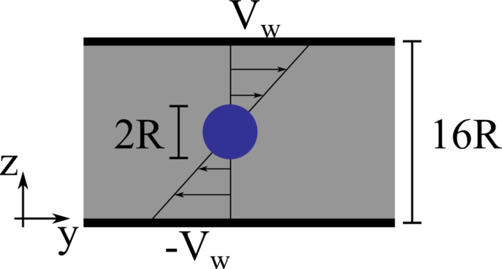
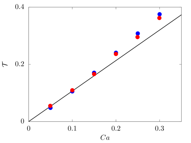
We consider a 3D spherical drop of radius \(R\) located at the center of a computational domain of size \(8R \times 16R \times 16R\), discretised with a resolution of \(20\) grid points per drop diameter. The top and bottom walls move with opposite velocity \(\pm V_w\), providing a shear rate \(\dot{\gamma} = 2 V_w/16R\), while periodic boundary conditions are imposed in the remaining directions. The same density and viscosity are specified for the spherical drop and the surrounding fluid, the Reynolds number \(Re = \rho \dot{\gamma} R^2/\mu\) is fixed to \(0.1\), and six capillary numbers are studied: \(0.05\), \(0.10\), \(0.15\), \(0.20\), \(0.25\) and \(0.30\).
config.h
#define _FLOW_COUETTE_
#define _SOLVER_FFT2D_
#define _MULTIPHASE_
#define _MULTIPHASE_VOF_
#define _MULTIPHASE_VOF_DROPLETS_
#define _MULTIPHASE_VISCOSITY_UNIFORM_
#define _MULTIPHASE_DENSITY_UNIFORM_
#define _MULTIPHASE_VOF_3D_
#define _MULTIPHASE_VOF_QUADRATIC_
param.f90
!Total number of grid points in X, Y and Z
integer, parameter :: nxt = 80, nyt = 160, nzt = 160
!Size of the domain in X, Y and Z
real, parameter :: lx = 4.0, ly = 8.0, lz = 8.0
!Fluid viscosity and density
real, parameter :: vis = 0.5**2/0.1, rho = 1.0
!Reference velocity (bulk velocity or wall velocity)
real, parameter :: refVel = 4.0
!Gravitational acceleration
real, dimension(3), parameter :: gr=(/0.0,0.0,-0.0/)
!Output frequency
integer,parameter :: iout0d = 100, iout1d = 100000, iout2d = 20000, iout3d = 100000, ioutfld = 100000
!Number of droplets
integer, parameter :: vofN = 1
!Interfacial surface tension
real, parameter :: vofSigma = vis*0.5/0.05
main.f90
! Simulation initial step
iStart = 0
! Simulation final step
iEnd = 9999999
! Choose the timestep
dt = 0.0001/2.0
initDropletPosition.dat
2.0 4.0 4.0 0.5
References:
[1] S. R. Hysing, S. Turek, D. Kuzmin, N. Parolini, E. Burman, S. Ganesan, and L. Tobiska. Quantitative benchmark computations of two-dimensional bubble dynamics. International Journal for Numerical Methods in Fluids, 60(11):1259-1288, 2009.
[2] S. Ii, K. Sugiyama, S. Takeuchi, S. Takagi, Y. Matsumoto, and F. Xiao. An interface capturing method with a continuous function: the THINC method with multi-dimensional reconstruction. Journal of Computational Physics, 231(5):2328–2358, 2012.
[3] G. I. Taylor. The formation of emulsions in definable fields of flow. Proceedings of the Royal Society of London A: Mathematical, Physical and Engineering Sciences, 146(858):501–523, 1934.
IBM - Rigid particle
Uniform flow around a cylinder
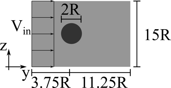
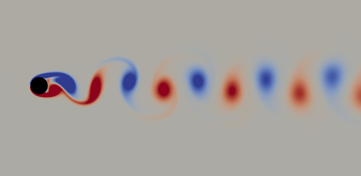
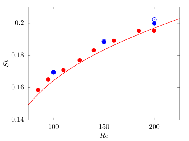
We consider a 2D rigid cylinder of radius R located in a computational domain of size \(15R \times 15R\), discretised with a resolution of \(68\) grid points per particle diameter. The incoming flow is uniform with velocity \(V_{in}\), providing a Reynolds number \(Re = D V_{in}/\nu\) of \(100\), \(150\) and \(200\).
config.h
#define _FLOW_COUETTE_
#define _FLOW_INOUT_
#define _FLOW_INOUT_UNBOUND_
#define _SOLVER_INOUT_
#define _MULTIPHASE_
#define _MULTIPHASE_IBM_
#define _MULTIPHASE_IBM_2D_
param.f90
! Total number of grid points in X, Y and Z
integer, parameter :: nxt = 4, nyt = 2048, nzt = 2048
! Size of the domain in X, Y and Z
real, parameter :: lx = 30.0/2048.*4., ly = 30.0, lz = 30.0
! Fluid viscosity and density
real, parameter :: vis = 1.0/200.0
real, parameter :: rho = 1.0
! Reference velocity (bulk velocity or wall velocity)
real, parameter :: refVel = 1.0
!Gravitational acceleration
real, dimension(3), parameter :: gr=(/0.0,0.0,-0.0/)
! Number of particles
integer, parameter :: ibmN = 1
! Particle radius and density
real, parameter :: ibmR = 0.5, ibmRho = 1.0, ibmRhoF = rho
input/input.in
# Simulation initial and final step
 1200000     9999999
 # Simulation time
 299.99999999463392
 # Simulation time-step
 2.5000000000000001E-004
 # Output frequency
 400     1000000       40000     1000000      400000
 # Simulation restart condition for the multiphase part
 F
initParticlePosition.dat
7.5 15.0
Lateral migration of a circular cylinder in a shear flow
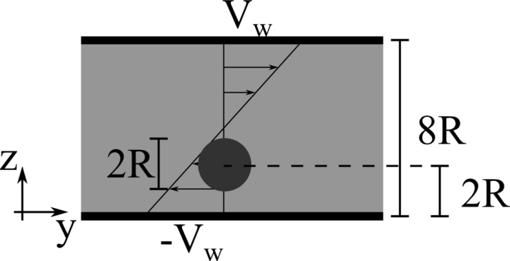
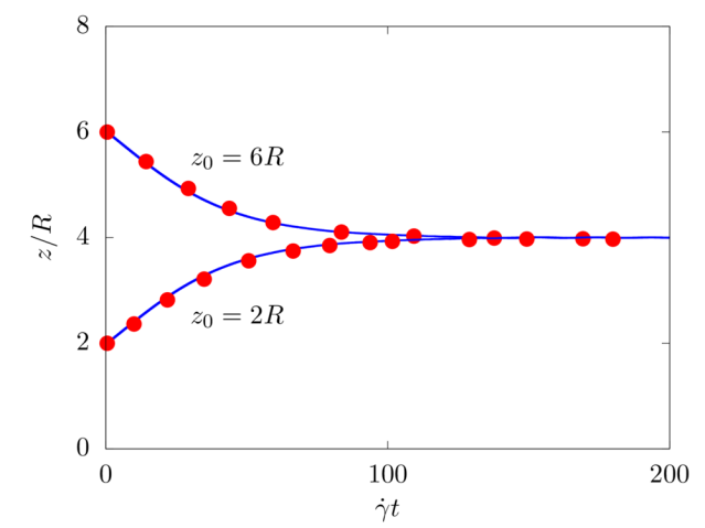
We consider a 2D rigid cylinder of radius R located in a computational domain of size \(8R \times 50R\), discretised with a resolution of \(16\) grid points per particle diameter. The top and bottom walls move with opposite velocity \(\pm V_w\), providing a shear rate \(\dot{\gamma} = 2 V_w/8R\), while periodic boundary conditions are imposed in the remaining directions. The particle is neutrally buoyant, and the Reynolds number \(Re = \rho \dot{\gamma} R^2 / \mu\) is fixed equal to \(40\). Two different initial conditions are studied: \(z = 2R\) and \(6R\).
config.h
#define _FLOW_COUETTE_
#define _SOLVER_FFT2D_
#define _MULTIPHASE_
#define _MULTIPHASE_IBM_
#define _MULTIPHASE_IBM_2D_
param.f90
!Total number of grid points in X, Y and Z
integer, parameter :: nxt = 4, nyt = 8*50, nzt = 8*8
!Size of the domain in X, Y and Z
real, parameter :: lx = 4.0/8.0, ly = 50.0, lz = 8.0
!Fluid viscosity and density
real, parameter :: vis = 1.0*8.0/40.0, rho = 1.0
!Reference velocity (bulk velocity or wall velocity)
real, parameter :: refVel = 0.5
!Gravitational acceleration
real, dimension(3), parameter :: gr=(/0.0,0.0,-0.0/)
!Output frequency
integer,parameter :: iout0d = 20, iout1d = 1000000, iout2d = 4000, iout3d = 1000000, ioutfld = 1000000
integer, parameter :: ibmN=1
real, parameter :: ibmR=1.0, ibmRhoF=rho, ibmRho=ibmRhoF, ibmVol=pi*ibmR**2, ibmMas=ibmRho*ibmVol, ibmIne=0.5*ibmMas*ibmR**2
main.f90
!Simulation initial step
iStart = 0
!Simulation final step
iEnd   = 9999999
!Choose the timestep
dt = 0.000001
initParticlePosition.dat
0.5 2.0
Lateral migration of a circular cylinder in a pressure driven flow
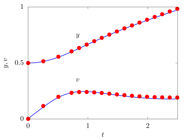
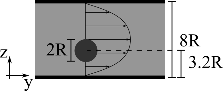
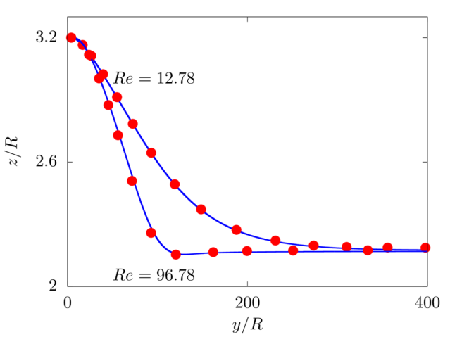
We consider a 2D rigid cylinder of radius R located in a computational domain of size \(8R \times 8R\), discretised with a resolution of \(32\) grid points per particle diameter. The flow is driven by an imposed pressure gradient, such that the resulting Reynolds number \(Re = \rho V_b 8R/\mu\) is equal to \(12.78\) and \(96.74\). The particle is neutrally buoyant and initially located at \(3.2R\) from the bottom wall.
config.h
#define _FLOW_CHANNEL_
#define _FLOW_CHANNEL_CPG_
#define _SOLVER_FFT2D_
#define _MULTIPHASE_
#define _MULTIPHASE_IBM_
#define _MULTIPHASE_IBM_2D_
param.f90
!Total number of grid points in X, Y and Z
integer, parameter :: nxt = 4, nyt = 256, nzt = 256
!Size of the domain in X, Y and Z
real, parameter :: lx = 1.0/128.0*4.0/2.0, ly = 1.0, lz = 1.0
!Fluid viscosity and density
real, parameter :: vis = 4.283E-04, rho = 1.0
!Reference velocity (bulk velocity or wall velocity)
real, parameter :: refVel = 0.0
!Imposed pressure gradient
real, parameter :: gradP = 2.337E-04
!Gravitational acceleration
real, dimension(3), parameter :: gr=(/0.0,0.0,-0.0/)
!Output frequency
integer,parameter :: iout0d = 20, iout1d = 1000000, iout2d = 4000, iout3d = 1000000, ioutfld = 1000000
integer, parameter :: ibmN=1
real, parameter :: ibmR=0.125, ibmRhoF=rho, ibmRho=ibmRhoF, ibmVol=pi*ibmR**2, ibmMas=ibmRho*ibmVol, ibmIne=0.5*ibmMas*ibmR**2
main.f90
!Simulation initial step
iStart = 0
!Simulation final step
iEnd   = 9999999
!Choose the timestep
dt = 0.001
initParticlePosition.dat
0.5 0.4
Sedimentation of a spherical particle
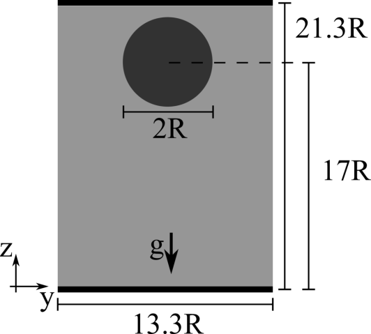
We consider a rectangular domain filled with a liquid with density and viscosity equal to \(960 kg~m^{−3}\) and \(0.058 Pa~s\). The domain size is \(0.1 m \times 0.1m \times 0.16m\) in the \(x\), \(y\) and \(z\) directions, where \(x\) and \(y\) are the two horizontal directions, while \(z\) is the vertical direction parallel to the gravitational acceleration \(g = 9.81 m~s^{-2}\). A particle of diameter \(0.015m\) and density \(1120 kg~m^{−3}\) is initially positioned at \(\left(0.05 m, 0.05 m, 0.1275 m \right)\).
config.h
#define _FLOW_CHANNEL_
#define _FLOW_CHANNEL_CPG_
#define _SOLVER_FFT2D_
#define _MULTIPHASE_
#define _MULTIPHASE_IBM_
#define _MULTIPHASE_IBM_3D_
param.f90
!Total number of grid points in X, Y and Z
integer, parameter :: nxt = 192, nyt = 192, nzt = 304
!Size of the domain in X, Y and Z
real, parameter :: lx = 0.1, ly = 0.1, lz = 0.1/192.0*304.0
!Fluid viscosity and density
real, parameter :: vis = 0.058, rho = 960.0
!Reference velocity (bulk velocity or wall velocity)
real, parameter :: refVel = 0.0
!Imposed pressure gradient
real, parameter :: gradP = 0.0
!Gravitational acceleration
real, dimension(3), parameter :: gr=(/0.0,0.0,-9.8/)
!Output frequency
integer,parameter :: iout0d = 20, iout1d = 1000000, iout2d = 1000000, iout3d = 1000000, ioutfld = 1000000
integer, parameter :: ibmN=1
real, parameter :: ibmR = 0.015/2.0, ibmRhoF = rho, ibmRho = 1120.0
main.f90
!Simulation initial step
iStart = 0
!Simulation final step
iEnd   = 9999999
!Choose the timestep
dt = 0.0001
initParticlePosition.dat
0.05 0.05 0.1275
References:
[1] C. H. K. Williamson. Defining a universal and continuous Strouhal-Reynolds number relationship for the laminar vortex shedding of a circular cylinder. Physics of Fluids, 31(10):2742–2744, 1988.
[2] E. Guilmineau and P. Queutey. A numerical simulation of vortex shedding from an oscillating circular cylinder. Journal of Fluids and Structures, 16(6):773–794, 2002.
[3] J. Feng, H. H. Hu, and D. D. Joseph. Direct simulation of initial value problems for the motion of solid bodies in a newtonian fluid. part 2. couette and poiseuille flows. Journal of Fluid Mechanics, 277:271–301, 1994.
[4] T. W. Pan and R. Glowinski. Direct simulation of the motion of neutrally buoyant circular cylinders in plane poiseuille flow. Journal of Computational Physics, 181(1):260–279, 2002.
[5] A. Ten Cate, C. H. Nieuwstad, J. J. Derksen, and H. E. A. Van den Akker. Particle imaging velocimetry experiments and lattice-boltzmann simulations on a single sphere settling under gravity. Physics of Fluids, 14(11):4012–4025, 2002.
IBM - Flexible fiber
Free vibration of unsupported and cantilevered fibers
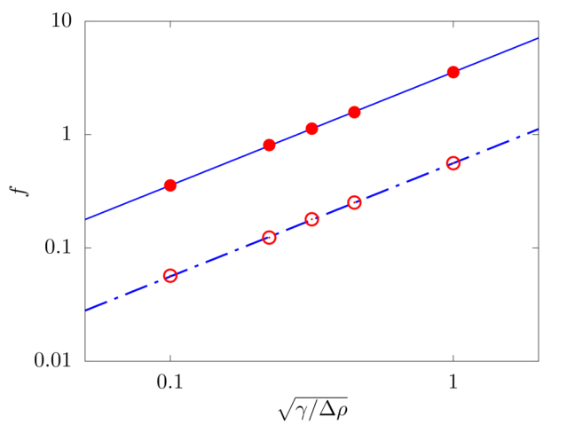
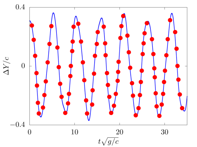
In the absence of any load, we evaulate the free vibration of a fiber. The filament length \(c\), flexibility \(\gamma\) and linear density difference \(\Delta \widetilde{\rho}\) are varied and the resulting frequency \(f\) of the free oscillations measured. The filament is discretised with \(100\) Lagrangian points.
Analytical solution - free: \(f = \frac{22.3733}{2 \pi c^2} \sqrt{\frac{\gamma}{\Delta \widetilde{\rho}}}\)
Analytical solution - clamped: \(f = \frac{3.5161}{2 \pi c^2} \sqrt{\frac{\gamma}{\Delta \widetilde{\rho}}}\)
config.h
#define _FLOW_CHANNEL_
#define _FLOW_FIXED_
#define _MULTIPHASE_
#define _MULTIPHASE_FIL_
#define _MULTIPHASE_FIL_FREE_
#define _MULTIPHASE_FIL_FIXD_
param.f90
! Gravitational acceleration
real, dimension(3), parameter :: gr=(/0.0,0.0,0.0/)
! Number of filaments
integer, parameter :: filN=1
! Number of Lagrangian points per filament
integer, parameter :: filNL=100
! Length of the filaments
real, parameter :: filL = 1.0
! Filament linear density difference and flexibility
real, parameter :: filDRhoL = 1.0, filGamma=0.01
input/input.in
# Simulation initial and final step
0     200000
# Simulation time
0.0
# Simulation time-step
1.0000000000000001E-004
# Output frequency
1     100000       100     1000000      1000000
# Simulation restart condition for the multiphase part
F
A hanging filament under gravity
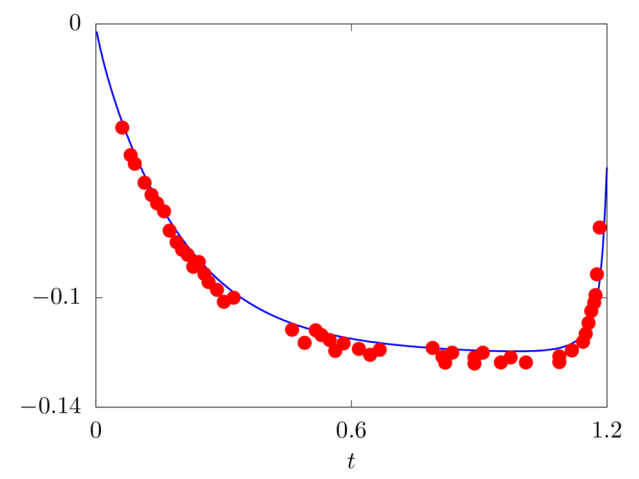
We consider the oscillations of a hanging filament under gravity. A filament of length \(c=1m\), linear density difference \(\Delta \widetilde{\rho}=1 kg/m\) and flexibility \(\gamma=0.01 kg~m^3 / s^2\) is initially held stationary with an angle of \(0.1 \pi\) from the vertical and then, after being released, starts swinging due to the gravity force \(g=10m/s^2\). The filament is discretised with \(100\) Lagrangian points.
config.h
#define _FLOW_CHANNEL_
#define _FLOW_FIXED_
#define _MULTIPHASE_
#define _MULTIPHASE_FIL_
#define _MULTIPHASE_FIL_HING_
#define _MULTIPHASE_FIL_FIXD_
param.f90
! Gravitational acceleration
real, dimension(3), parameter :: gr=(/0.0,10.0,0.0/)
! Number of filaments
integer, parameter :: filN=1
! Number of Lagrangian points per filament
integer, parameter :: filNL=100
! Length of the filaments
real, parameter :: filL = 1.0
! Filament linear density difference and flexibility
real, parameter :: filDRhoL = 1.0, filGamma=0.01
input/input.in
# Simulation initial and final step
0     200000
# Simulation time
0.0
# Simulation time-step
1.0000000000000001E-004
# Output frequency
1     100000       100     1000000      1000000
# Simulation restart condition for the multiphase part
F
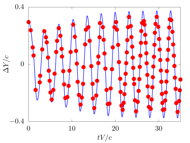
A hanging filament in a uniform flow
We consider the oscillations of a hanging filament in a uniform flow with velocity \(V\). A filament of length \(c=1m\), linear density difference \(\Delta \widetilde{\rho}=1.5 kg/m\) and flexibility \(\gamma=0.0015 kg~m^3 / s^2\) is initially held stationary with an angle of \(0.1 \pi\) from the vertical and then, after being released, starts swinging due to the combined effect of the viscous fluid flow (\(\nu=0.005m^2/s\)) and gravity force (\(g=0.5m/s^2\)). The filament is discretised with \(65\) Lagrangian points.
config.h
#define _FLOW_INOUT_
#define _FLOW_INOUT_UNBOUND_
#define _SOLVER_INOUT_
#define _MULTIPHASE_
#define _MULTIPHASE_IBML_
#define _MULTIPHASE_IBML_GLDS_
#define _MULTIPHASE_IBML_GLDS_2D_
#define _MULTIPHASE_IBML_XXXX_READ_
#define _MULTIPHASE_IBML_XXXX_FIL_
#define _MULTIPHASE_IBML_XXXX_FIL_HING_
param.f90
! Fluid viscosity and density
real, parameter :: vis = 1.0/200.0
real, parameter :: rho = 1.0
! Reference velocity (bulk velocity or wall velocity)
real, parameter :: refVel = 1.0
! Gravitational acceleration
real, dimension(3), parameter :: gr=(/0.0,0.5,0.0/)
! Number of objects
integer, parameter :: ibmlN=1
! Number of Lagrangian points per object
integer, parameter :: ibmlNL=65
! Linear dimension of the object
real, parameter :: ibmlL = 1.0
! Moving or not object
logical, parameter ::  ibmlMoving = .TRUE.
! Filament linear density difference and flexibility
real, parameter :: filDRhoL = 1.5, filGamma=1e-3*filDRhoL
input/input.in
# Simulation initial and final step
0       100000
# Simulation time
0.0
# Simulation time-step
5.0E-004
# Output frequency: 0D, 1D, 2D, 3D, restart data
100       10000        100000     1000000      2000000
# Simulation restart condition for the multiphase part
F
References:
[1] W. X. Huang, S. J. Shin, and H. J. Sung. Simulation of flexible filaments in a uniform flow by the immersed boundary method. Journal of Computational Physics, 226(2):2206–2228, 2007.
Non-Newtonian fluid
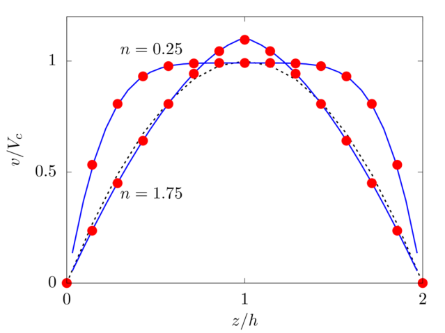
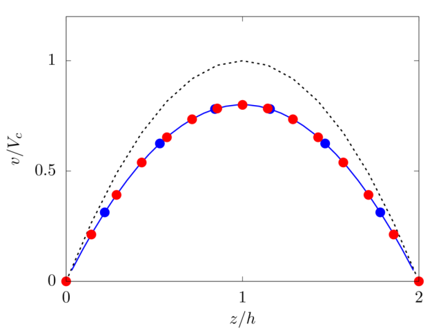
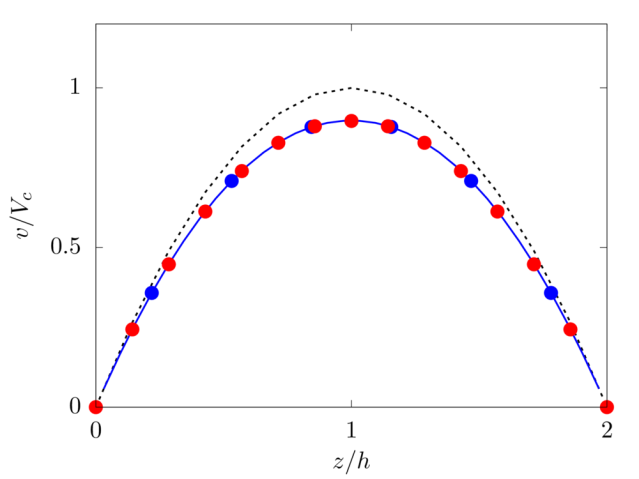
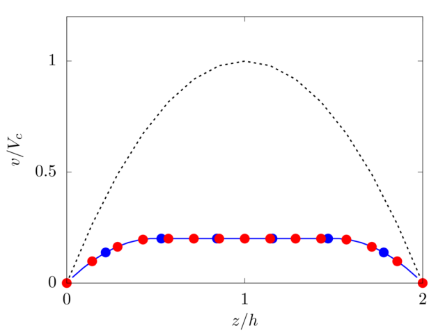
We consider the pressure-driven flow of a viscous fluid in a channel, i.e., a plane Poiseuille flow. \(x\), \(y\), and \(z\) denote the spanwise, streamwise, and wall-normal coordinates, while \(u\), \(v\), and \(w\) the corresponding components of the velocity vector field. The lower and upper impermeable walls are located at \(z=-h\) and \(z=h\), respectively, and the flow is driven by a uniform pressure gradient in the streamwise direction \(P_y\). The pressure gradient is such that with a Newtonian fluid the centerline velocity \(V_c = P_y h^2/2 \mu\) is equal to \(1\). \(32\) grid points are used to discretise the domain in the wall-normal direction. Different non-Newtonian fluids are considered.
Power-law fluid
We consider shear-thinning and thickening fluids modeled as simple power-law fluids with local viscosity \(\mu_l = k \dot{\gamma}^{n-1}\), with power index \(n=0.75\) and \(1.75\), respectively, and fluid consistency index \(k\) such that \(\mu_l \left( \dot{\gamma}_0 \right)= \mu\), being \(\dot{\gamma}_0\) the mean shear rate in the channel for a Newtonian fluid, i.e. \(P_y/2 \mu h\).
Analytical solution: \(v \left( z \right) = \frac{n}{n+1} \left( \frac{P_y}{k}\right)^{\frac{1}{n}} \left[ h^\frac{n+1}{n} - \left(z-h\right)^\frac{n+1}{n} \right]\).
config.h
#define _FLOW_CHANNEL_
#define _FLOW_CHANNEL_CPG_
#define _FLOW_CHANNEL_LAMINAR_
#define _SOLVER_FFT2D_
#define _MULTIPHASE_
#define _MULTIPHASE_NNF_
#define _MULTIPHASE_VISCOSITY_VARIABLE_
#define _MULTIPHASE_DENSITY_UNIFORM_
#define _MULTIPHASE_NNF_POW_
#define _MULTIPHASE_NNF_POW_C_
param.f90
! Total number of grid points in X, Y and Z
integer, parameter :: nxt = 4, nyt = 4, nzt = 32
! Size of the domain in X, Y and Z
real, parameter :: lx = 0.25, ly = 0.25, lz = 2.0
! Fluid viscosity and density
real, parameter :: vis = 0.01, rho = 1.0
! Imposed pressure gradient
real, parameter :: gradP = 0.02
! Reference velocity (bulk velocity or wall velocity)
real, parameter :: refVel = gradP/(3.0*vis)
! Gravitational acceleration
real, dimension(3), parameter :: gr=(/0.0,0.0,0.0/)
! Output frequency
integer,parameter :: iout0d = 100000, iout1d = 100000, iout2d = 10000000, iout3d = 10000000, ioutfld = 10000000
! Power-law index
real, parameter :: nn_n = 1.75 !THICK: 1.75 - THIN: 0.75
! Fluid consistency index
real, parameter :: nn_k=vis*(3.0*refVel/lz)**(1.0-nn_n)
main.f90
! Simulation initial step
iStart = 0
! Simulation final step
iEnd = 1000000
! Choose the timestep
dt = 0.0002
Oldroyd-B fluid
We consider an Oldroyd-B fluid [1] with relaxation time \(\lambda = 10\) and polymeric viscossity \(\mu_p=\mu/4\).
Analytical solution: \(v \left( z \right) = 2 P_y h^2/ \left( \mu+\mu_p \right) \left( z/2h \right)\left[ 1- \left( z/2h \right) \right]\).
config.h
#define _FLOW_CHANNEL_
#define _FLOW_CHANNEL_CPG_
#define _FLOW_CHANNEL_LAMINAR_
#define _SOLVER_FFT2D_
#define _MULTIPHASE_
#define _MULTIPHASE_NNF_
#define _MULTIPHASE_VISCOSITY_UNIFORM_
#define _MULTIPHASE_DENSITY_UNIFORM_
#define _MULTIPHASE_NNF_OLB_
param.f90
! Total number of grid points in X, Y and Z
integer, parameter :: nxt = 4, nyt = 4, nzt = 32
! Size of the domain in X, Y and Z
real, parameter :: lx = 0.25, ly = 0.25, lz = 2.0
! Fluid viscosity and density
real, parameter :: vis = 0.01, rho = 1.0
! Imposed pressure gradient
real, parameter :: gradP = 0.02
! Reference velocity (bulk velocity or wall velocity)
real, parameter :: refVel = gradP/(3.0*vis)
! Gravitational acceleration
real, dimension(3), parameter :: gr=(/0.0,0.0,0.0/)
! Output frequency
integer,parameter :: iout0d = 100000, iout1d = 100000, iout2d = 10000000, iout3d = 10000000, ioutfld = 10000000
! Polymeric viscosity and relaxation time
real, parameter :: nnVis=vis/4.0, nnLambda=10.0
main.f90
! Simulation initial step
iStart = 0
! Simulation final step
iEnd = 2000000
! Choose the timestep
dt = 0.0002
FENE-P fluid
We consider a FENE-P fluid [2] with relaxation time \(\lambda=10\), polymeric viscosity \(\mu_p=\mu/4\) and maximum dumbbell extension \(L=6\).
Analytical solution [3]: \(u= 2 P_y h^2/\mu \left( z/2h \right)\left[ 1- \left( z/2h \right) \right] + 3/(8 C \mu) (A_+^{1/3} B_- - C_+^{1/3} D_- + A_-^{1/3} B_+ - C_-^{1/3} D_+)\),
where
\(A_\pm = Bh \pm \sqrt{B^2h^2 + A^3}\),
\(B_\pm = 3Bh \pm \sqrt{B^2h^2 + A^3}\),
\(C_\pm = B \left( z-1\right) \pm \sqrt{B^2\left( z-1\right)^2 + A^3}\),
\(D_\pm = 3 B \left( z-1\right) \pm \sqrt{B^2 \left( z-1\right)^2 + A^3}\),
with
config.h
#define _FLOW_CHANNEL_
#define _FLOW_CHANNEL_CPG_
#define _FLOW_CHANNEL_LAMINAR_
#define _SOLVER_FFT2D_
#define _MULTIPHASE_
#define _MULTIPHASE_NNF_
#define _MULTIPHASE_VISCOSITY_UNIFORM_
#define _MULTIPHASE_DENSITY_UNIFORM_
#define _MULTIPHASE_NNF_FEN_
param.f90
! Total number of grid points in X, Y and Z
integer, parameter :: nxt = 4, nyt = 4, nzt = 32
! Size of the domain in X, Y and Z
real, parameter :: lx = 0.25, ly = 0.25, lz = 2.0
! Fluid viscosity and density
real, parameter :: vis = 0.01, rho = 1.0
! Imposed pressure gradient
real, parameter :: gradP = 0.02
! Reference velocity (bulk velocity or wall velocity)
real, parameter :: refVel = gradP/(3.0*vis)
! Gravitational acceleration
real, dimension(3), parameter :: gr=(/0.0,0.0,0.0/)
! Output frequency
integer,parameter :: iout0d = 100000, iout1d = 100000, iout2d = 10000000, iout3d = 10000000, ioutfld = 10000000
! Polymeric viscosity and relaxation time
real, parameter :: nnVis=vis/4.0, nnLambda=10.0
! FENE-P dumbbell extensibility
real, parameter :: nnL2=6.0**2
main.f90
! Simulation initial step
iStart = 0
! Simulation final step
iEnd = 2000000
! Choose the timestep
dt = 0.0002
Elastoviscoplatic fluid
We consider an elastoviscoplastic fluid modelled with the Saramito model [4]. We fix the relaxation time \(\lambda=0.01\), polymeric viscosity \(\mu_p=\mu/4\) and yield stress \(\tau_0 = 0.01\). Due to the low value of \(\lambda\) considered, we compare the result with the purely viscoplastic solution.
Analytical solution: \(v \left( z \right) = P_y/2 \left( \mu + \mu_p \right) \left[ (z-1)^2 - h^2 \right] + \tau_0/ \left( \mu + \mu_p \right) \left[ (z-1) -h \right]\) if \(z_0 \le z-1 \lt h\) else \(v \left( z \right) = v \left( z_0+1 \right)\).
config.h
#define _FLOW_CHANNEL_
#define _FLOW_CHANNEL_CPG_
#define _FLOW_CHANNEL_LAMINAR_
#define _SOLVER_FFT2D_
#define _MULTIPHASE_
#define _MULTIPHASE_NNF_
#define _MULTIPHASE_VISCOSITY_UNIFORM_
#define _MULTIPHASE_DENSITY_UNIFORM_
#define _MULTIPHASE_NNF_EVP_
param.f90
! Total number of grid points in X, Y and Z
integer, parameter :: nxt = 4, nyt = 4, nzt = 32
! Size of the domain in X, Y and Z
real, parameter :: lx = 0.25, ly = 0.25, lz = 2.0
! Fluid viscosity and density
real, parameter :: vis = 0.01, rho = 1.0
! Imposed pressure gradient
real, parameter :: gradP = 0.02
! Reference velocity (bulk velocity or wall velocity)
real, parameter :: refVel = gradP/(3.0*vis)
! Gravitational acceleration
real, dimension(3), parameter :: gr=(/0.0,0.0,0.0/)
! Output frequency
integer,parameter :: iout0d = 100000, iout1d = 100000, iout2d = 10000000, iout3d = 10000000, ioutfld = 10000000
! Polymeric viscosity and relaxation time
real, parameter :: nnVis=vis/4.0, nnLambda=10.0/1000.0
! Yield stress (tautau0 fluid-like behaviour)
real, parameter :: nnTau0=0.01
main.f90
! Simulation initial step
iStart = 0
! Simulation final step
iEnd = 2000000
! Choose the timestep
dt = 0.0002
Steady and periodic shear flow with EVP fluid
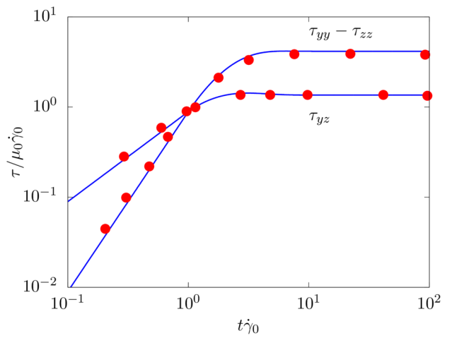
First, we consider a simple constant shear flow, with the shear rate \(\dot{\gamma}_0\): the Weissenberg number is fixed to \(Wi = \lambda \dot{\gamma}_0 = 1\), the Bingham number \(Bi = \tau_0 / \left[ \left( \mu+\mu_p \right) \dot{\gamma}_0 \right] = 1\), and the viscosity ratio \(\beta = \mu / \left( \mu + \mu_p \right) =1/9\).
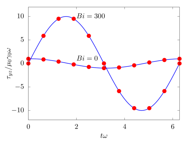
Next, we consider a time-periodic uniform shear flow, i.e. \(\gamma_0 \sin \left( \omega_0 t \right)\), where \(\gamma_0\) is the strain amplitude and \(\omega_0\) the angular frequency of the oscillations. The Weissenberg number is \(Wi = \lambda \omega_0 = 0.1\) and two Bingham numbers \(Bi = \tau_0/\left[ \left( \mu + \mu_p \right) \gamma_0 \omega_0 \right]\) are considered: \(Bi = 0\) and \(300\). Note that, when \(Bi = 0\), the material behaves like a viscoelastic fluid, and when \(Bi = 300\) as an elastic solid. The viscosity ratio \(\beta = \mu / \left( \mu + \mu_p \right)\) is null in both cases, i.e. \(\mu = 0\).
config.h
#define _FLOW_CHANNEL_
#define _FLOW_FIXED_
#define _SOLVER_FFT2D_
#define _MULTIPHASE_
#define _MULTIPHASE_NNF_
#define _MULTIPHASE_VISCOSITY_UNIFORM_
#define _MULTIPHASE_DENSITY_UNIFORM_
#define _MULTIPHASE_NNF_EVP_
param.f90
! Total number of grid points in X, Y and Z
integer, parameter :: nxt = 4, nyt = 64, nzt = 64
! Size of the domain in X, Y and Z
real, parameter :: lx = 1.0, ly = 1.0, lz = 1.0
! Fluid viscosity and density
real, parameter :: vis = 0.0, rho = 1.0 !Steady: 1.0/9.0, 1.0 - Oscillating: 0.0, 1.0
! Reference velocity (bulk velocity or wall velocity)
real, parameter :: refVel = 0.5
! Gravitational acceleration
real, dimension(3), parameter :: gr=(/0.0,0.0,0.0/)
! Output frequency
integer,parameter :: iout0d = 10, iout1d = 10000000, iout2d = 10000000, iout3d = 10000000, ioutfld = 10000000
! Polymeric viscosity and relaxation time
real, parameter :: nnVis=1.0, nnLambda=0.1 !Steady: 8.0/9.0, 1.0 - Oscillating: 1.0, 0.1
! Yield stress (tautau0 fluid-like behaviour)
real, parameter :: nnTau0=300.0 !Steady: 1.0 - Oscillating: 0.0/300.0
main.f90
! Simulation initial step
iStart = 0
! Simulation final step
iEnd = 1000000
! Choose the timestep
dt = 0.001
References:
[1] J. G. Oldroyd. On the formulation of rheological equations of state. In Proceedings of the Royal Society of London A: Mathematical, Physical and Engineering Sciences, volume 200, pages 523–541. The Royal Society, 1950.
[2] A. Peterlin. Hydrodynamics of macromolecules in a velocity field with longitudinal gradient. Journal of Polymer Science: Polymer Letters, 4(4):287–291, 1966.
[3] D. O. A. Cruz, F. Pinho, and P. J. Oliveira. Analytical solutions for fully developed laminar flow of some viscoelastic liquids with a newtonian solvent contribution. Journal of Non-Newtonian Fluid Mechanics, 132(1-3):28–35, 2005.
[4] P. Saramito. A new constitutive equation for elastoviscoplastic fluid flows. Journal of Non-Newtonian Fluid Mechanics, 145(1):1–14, 2007.
Non-Newtonian multiphase flow
Rotation of a spherical particle in a Non-Newtonian Couette flow
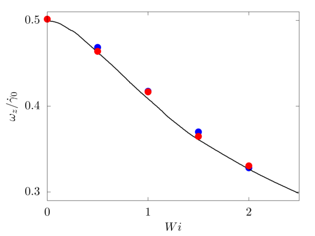
We consider a spherical particle of radius \(R\) immersed in a Non-Newtonian elastic fluid. The computational domain has size \(4 R \times 8R \times 8R\) and is discretised with \(24\) grid points per particle diameter. The top and bottom walls move with opposite velocity \(\pm V_w\), providing a shear rate \(\dot{\gamma} = 2V_w/8R\), while periodic boundary conditions are imposed in the remaining directions. The particle is neutrally buoyant, and the Reynolds number \(Re = \rho \dot{\gamma} R^2 / \mu\) is fixed equal to \(0.025\). The fluid is modelled with the Oldroyd-B model and the Weissenberg number \(Wi = \lambda \dot{\gamma}\) is varied between \(0\) and \(2\).
config.h
#define _FLOW_COUETTE_
#define _SOLVER_FFT2D_
#define _MULTIPHASE_
#define _MULTIPHASE_NNF_
#define _MULTIPHASE_IBM_
#define _MULTIPHASE_VISCOSITY_UNIFORM_
#define _MULTIPHASE_DENSITY_UNIFORM_
#define _MULTIPHASE_NNF_OLB_
#define _MULTIPHASE_NNF_XXX_LOG_
#define _MULTIPHASE_IBM_3D_
param.f90
!Total number of grid points in X, Y and Z
integer, parameter :: nxt = 24*2, nyt = 24*4, nzt = 24*4
!Size of the domain in X, Y and Z
real, parameter :: lx = 2.0, ly = 4.0, lz = 4.0
!Fluid viscosity and density
real, parameter :: vis = 5.0, rho = 1.0
!Reference velocity (bulk velocity or wall velocity)
real, parameter :: refVel = 1.0
!Gravitational acceleration
real, dimension(3), parameter :: gr=(/0.0,0.0,-0.0/)
!Output frequency
integer,parameter :: iout0d = 500, iout1d = 1000000, iout2d = 1000000, iout3d = 1000000, ioutfld = 1000000
real, parameter :: nnVis=vis, nnLambda=4.0
integer, parameter :: ibmN=1
real, parameter :: ibmR = 0.5, ibmRho = rho, ibmRhoF = rho
main.f90
!Simulation initial step
iStart = 0
!Simulation final step
iEnd   = 9999999
!Choose the timestep
dt = 0.000001*32./24.
initPositionParticle.dat
1.0 2.0 2.0 0.5
References:
[1] F. Snijkers, G. D’Avino, P. L. Maffettone, F. Greco, M. A. Hulsen, and J. Vermant. Effect of vis- coelasticity on the rotation of a sphere in shear flow. Journal of Non-Newtonian Fluid Mechanics, 166(7-8):363–372, 2011.
[2] N. Goyal and J. J. Derksen. Direct simulations of spherical particles sedimenting in viscoelastic fluids. Journal of Non-Newtonian Fluid Mechanics, 183:1–13, 2012.


